import numpy as np
import matplotlib.pyplot as plt
import scipy as sp
import statsmodels.formula.api as smf
import linregfunc as lr
import pandas as pd
import seaborn as sns

plt.style.use("fivethirtyeight")
Here we will have a quick refresh of distributions that are commonly used in hypothesis testing.
The Normal Distributions
Normal Distribution is the most important one among all, here we provide a graphic reminder of bivariate normal distribution. Please check out my notebooks of linear algebra, there is a whole chapter devoted for normal distribution.
For your reference, the pdf of multivariate normal distribution is
\[ p(\boldsymbol{x} ; \mu, \Sigma)=\frac{1}{(2 \pi)^{n / 2}|\Sigma|^{1 / 2}} \exp \left(-\frac{1}{2}(x-\mu)^{T} \Sigma^{-1}(x-\mu)\right) \]
x = np.linspace(-10, 10, 500)
y = np.linspace(-10, 10, 500)
X, Y = np.meshgrid(x, y)

pos = np.array([X.flatten(), Y.flatten()]).T  # two columns matrix

fig = plt.figure(figsize=(14, 14))

#########################
ax = fig.add_subplot(221, projection="3d")

mu_x = 0
mu_y = 0

sigma_x = 3
sigma_y = 15
rho = 3

rv = sp.stats.multivariate_normal(
    [mu_x, mu_y], [[sigma_x, rho], [rho, sigma_y]]
)  # frozen distribution
ax.plot_surface(X, Y, rv.pdf(pos).reshape(500, 500), cmap="coolwarm")

ax = fig.add_subplot(223)
ax.contour(rv.pdf(pos).reshape(500, 500))
string1 = r"$\sigma_x = %.1f$, $\sigma_y = %.1f$, $\rho = %.1f$" % (
    sigma_x,
    sigma_y,
    rho,
)
ax.annotate(text=string1, xy=(0.2, 0.05), xycoords="axes fraction", color="r")

####

mu_x = 0
mu_y = 0

sigma_x = 10
sigma_y = 4
rho = 0

rv = sp.stats.multivariate_normal(
    [mu_x, mu_y], [[sigma_x, rho], [rho, sigma_y]]
)  # frozen distribution
ax = fig.add_subplot(222, projection="3d")
ax.plot_surface(X, Y, rv.pdf(pos).reshape(500, 500), cmap="coolwarm")

ax = fig.add_subplot(224)
ax.contour(rv.pdf(pos).reshape(500, 500))
string2 = r"$\sigma_x = %.1f$, $\sigma_y = %.1f$, $\rho = %.1f$" % (
    sigma_x,
    sigma_y,
    rho,
)
ax.annotate(text=string2, xy=(0.2, 0.05), xycoords="axes fraction", color="r")
#########################

plt.show()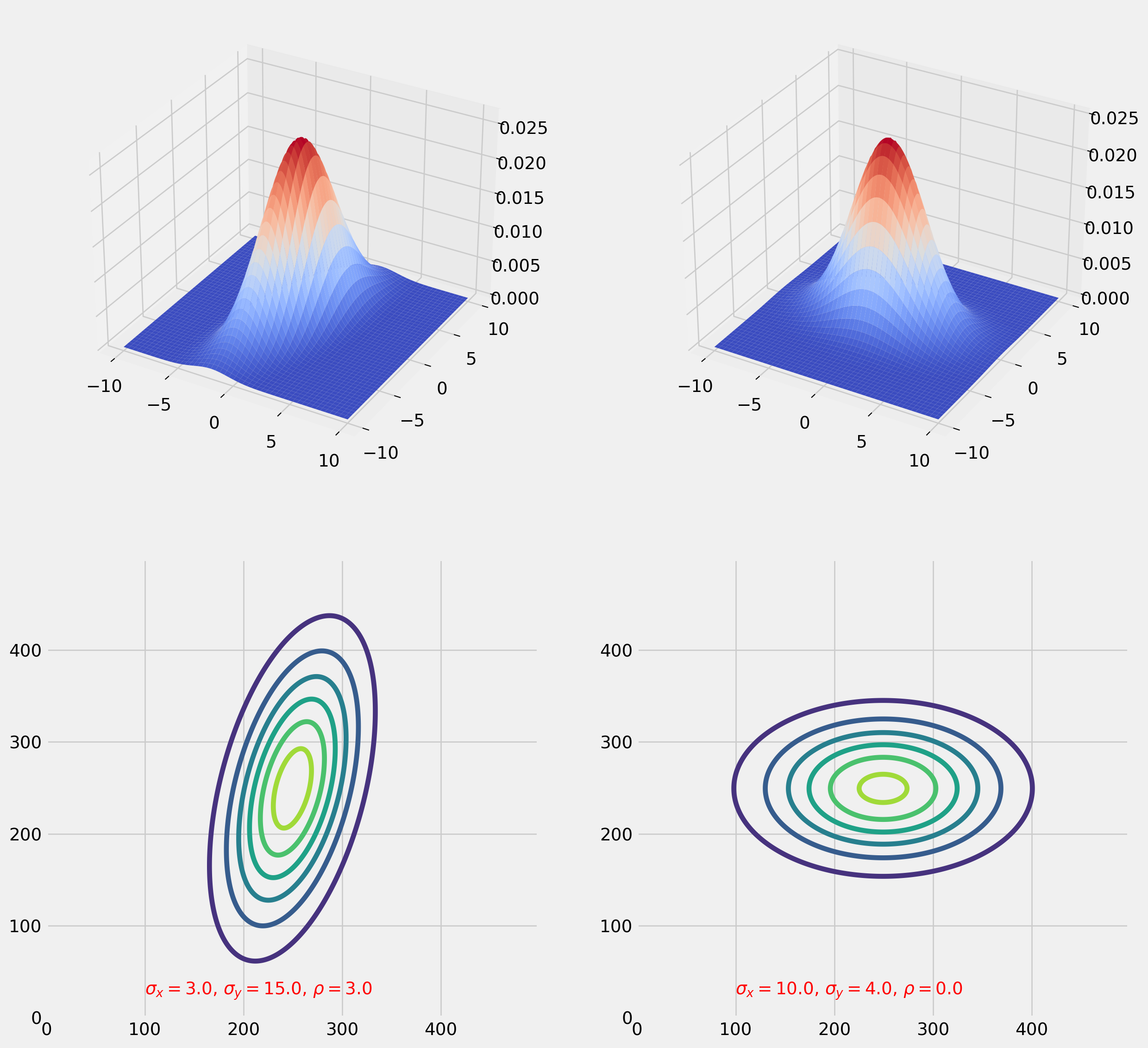
Keep in your mind: any linear combination of normally distributed variables is yet a normal distribution.
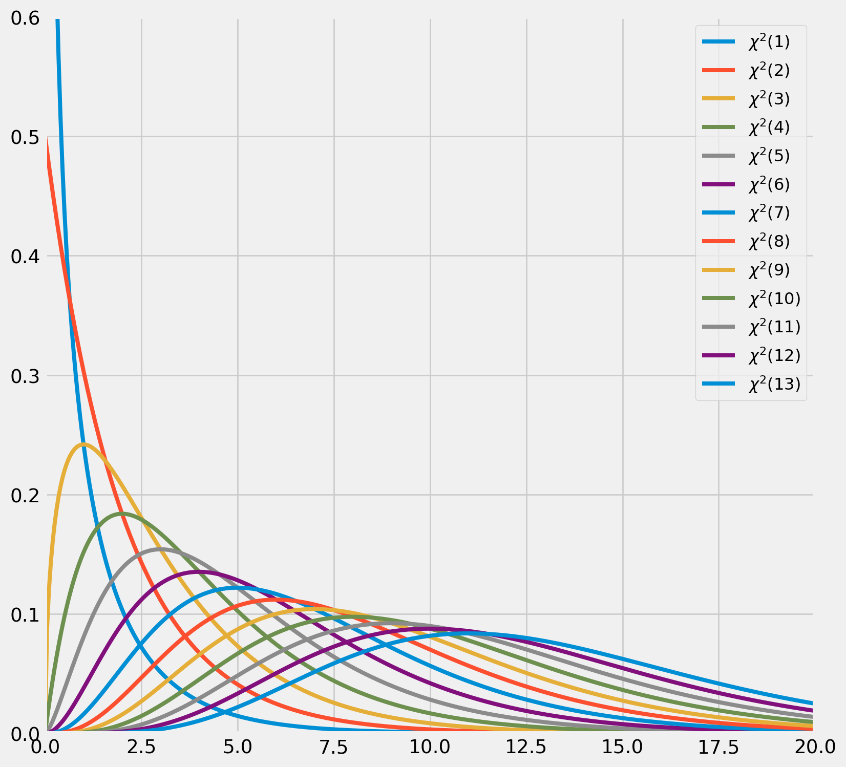
The Chi-Squared Distribution
If an \(n\)-random vector follows \(iid\) normal distribution, \(\boldsymbol{z}\sim N(\boldsymbol{0}, \mathbf{I})\). Then the random variable
\[ y = \boldsymbol{z}^T\boldsymbol{z} = \sum_{i=i}^n z_i^2 \]
is said to follow the chi-squared distribution with \(n\) degrees of freedom. Denoted as
\[ y\sim\chi^2(n) \]
The mean is
\[\mathrm{E}(y)=\sum_{i=1}^{m} \mathrm{E}\left(z_{i}^{2}\right)=\sum_{i=1}^{m} 1=m\]
And the variance is
\[\begin{aligned} \operatorname{Var}(y) &=\sum_{i=1}^{m} \operatorname{Var}\left(z_{i}^{2}\right)=m \mathrm{E}\left(\left(z_{i}^{2}-1\right)^{2}\right) \\ &=m \mathrm{E}\left(z_{i}^{4}-2 z_{i}^{2}+1\right)=m(3-2+1)=2 m \end{aligned}\]
As \(n\) increases, the probability density function of \(\chi^2\) approaches the \(N(m, 2m)\). Here is the graphic demonstration shows how \(\chi^2\) distribution changes as d.o.f. rises.
fig, ax = plt.subplots(figsize=(9, 9))
x = np.linspace(0, 50, 1000)
for i in range(1, 14):
    chi_pdf = sp.stats.chi2.pdf(x, i)
    ax.plot(x, chi_pdf, lw=3, label="$\chi^2 (%.0d)$" % i)
    ax.legend(fontsize=12)
ax.axis([0, 20, 0, 0.6])
plt.show()
<>:5: SyntaxWarning:
invalid escape sequence '\c'
<>:5: SyntaxWarning:
invalid escape sequence '\c'
/tmp/ipykernel_2979/3312535410.py:5: SyntaxWarning:
invalid escape sequence '\c'
Quadratic Form of \(\chi^2\) Distribution
If an \(n\)-random vector \(\boldsymbol{y} \sim N(\boldsymbol{\mu}, \Sigma)\) then
\[ (\boldsymbol{y} - \boldsymbol{\mu})^T\Sigma^{-1}(\boldsymbol{y}-\boldsymbol{\mu})\sim \chi^2(n) \]
If \(\boldsymbol{y} \sim N(\boldsymbol{0}, \Sigma)\) simplifies the expression
\[ \boldsymbol{y}^T\Sigma^{-1}\boldsymbol{y}\sim \chi^2(n) \]
We will show why that holds by using diagonal decomposition. Since the \(\Sigma\) is symmetric, it is orthogonally diagonalizable,
\[ \Sigma = QDQ^T \]
where
\[ D=\left[\begin{array}{ccccc} \lambda_{1} & 0 & 0 & \ldots & 0 \\ 0 & \lambda_{2} & 0 & \ldots & 0 \\ \vdots & \vdots & \vdots & & \vdots \\ 0 & 0 & 0 & \ldots & \lambda_{n} \end{array}\right] \]
\(\lambda\)s are eigenvalues. And \(Q^{-1} = Q^T\), \(Q\) holds all the eigenvectors of \(\Sigma\) which are mutually perpendicular.
Denote \(D^*\) as
\[ D^* = \left[\begin{array}{ccccc} \frac{1}{\sqrt{\lambda_{1}}} & 0 & 0 & \ldots & 0 \\ 0 & \frac{1}{\sqrt{\lambda_{2}}} & 0 & \ldots & 0 \\ \vdots & \vdots & \vdots & & \vdots \\ 0 & 0 & 0 & \ldots & \frac{1}{\sqrt{\lambda_{n}}} \end{array}\right] \]
Let the matrix \(H = QD^*Q^T\), since \(H\) is also symmetric
\[ HH^T= QD^*Q^TQD^*Q^T= Q^TD^*D^*Q = QD^{-1}Q^T =\Sigma^{-1} \]
Furthermore
\[ H\Sigma H^T = QD^*Q^T\Sigma QD^*Q^T = QD^*Q^TQDQ^T QD^*Q^T = QD^*DD^*Q^T = QQ^T = I \]
Back to the results from above, we set \(\boldsymbol{z} = H^T (\boldsymbol{y}-\boldsymbol{\mu})\), which is standard normal distribution since
\[ E(\boldsymbol{z})= H^TE(\boldsymbol{y}-\boldsymbol{\mu})=\boldsymbol{0}\\ \text{Var}(\boldsymbol{z}) = H\text{Var}(\boldsymbol{y}-\boldsymbol{\mu})H^T =H\Sigma H^T = I \]
Back to where we started
\[ (\boldsymbol{y}-\boldsymbol{\mu})^T\Sigma^{-1}(\boldsymbol{y}-\boldsymbol{\mu}) = (\boldsymbol{y}-\boldsymbol{\mu})^THH^T (\boldsymbol{y}-\boldsymbol{\mu}) = (H^T (\boldsymbol{y}-\boldsymbol{\mu}))^T(H^T (\boldsymbol{y}-\boldsymbol{\mu})) = \boldsymbol{z}^T\boldsymbol{z} \]
here we proved that \((\boldsymbol{y}-\boldsymbol{\mu})^T\Sigma^{-1}(\boldsymbol{y}-\boldsymbol{\mu}) \sim \chi^2(n)\).
More details of proof in this page.
The Student’s \(t\) Distribution
If \(z\sim N(0, 1)\) and \(y\sim \chi^2(m)\), and \(z\) and \(y\) are independent, then
\[ t = \frac{z}{\sqrt{y/m}} \]
follows the Student’s t distribution with \(m\) d.o.f.
Here is the plot of \(t\)-distribution, note that \(t(1)\) is called Cauchy distribution which has no moments at all, because integral does not converge due to fat tails.
fig, ax = plt.subplots(figsize=(12, 7))
x = np.linspace(-5, 5, 1000)
for i in range(1, 6):
    chi_pdf = sp.stats.t.pdf(x, i)
    if i == 1:
        ax.plot(x, chi_pdf, lw=3, label="Cauchy", ls="--")
        continue
    else:
        ax.plot(x, chi_pdf, lw=3, label="$t (%.0d)$" % i)
        ax.legend(fontsize=12)
ax.axis([-5, 5, 0, 0.4])
ax.set_title("Student's $t$ Distribution", size=18)
plt.show()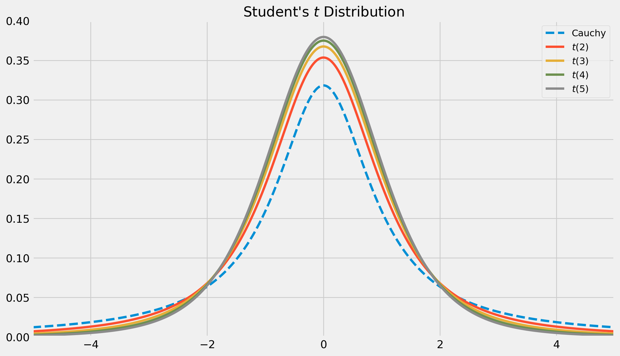
As \(m \rightarrow \infty\), \(t(m)\rightarrow N(0, 1)\), in the limit process, the tails of \(t\) distribution will diminish, and becoming thinner.
The \(F\) Distribution
If \(y_1\) and \(y_2\) are independent random variables distributed as \(\chi^2(m_1)\) and \(\chi^2(m_2)\), then the random variable
\[ F = \frac{y_1/m_1}{y_2/m_2} \]
follows the \(F\) distribution, denoted $ F(m_1, m_2)$.
x = np.linspace(0.001, 5, 100)
fig, ax = plt.subplots(figsize=(12, 7))

df1 = 10
df2 = 2
f_pdf = sp.stats.f.pdf(x, dfn=df1, dfd=df2)
ax.plot(x, f_pdf, lw=3, label="$df_1 = %.d, df_2 = %.d$" % (df1, df2))

df1 = 2
df2 = 10
f_pdf = sp.stats.f.pdf(x, dfn=df1, dfd=df2)
ax.plot(x, f_pdf, lw=3, label="$df_1 = %.d, df_2 = %.d$ " % (df1, df2))

df1 = 8
df2 = 15
f_pdf = sp.stats.f.pdf(x, dfn=df1, dfd=df2)
ax.plot(x, f_pdf, lw=3, color="red", label="$df_1 = %.d, df_2 = %.d$" % (df1, df2))

df1 = 15
df2 = 8
f_pdf = sp.stats.f.pdf(x, dfn=df1, dfd=df2)
ax.plot(x, f_pdf, lw=3, label="$df_1 = %.d, df_2 = %.d$ " % (df1, df2))

ax.legend(fontsize=15)
ax.axis([0, 4, 0, 0.8])
ax.set_title("$F$ Distribution", size=18)
plt.show()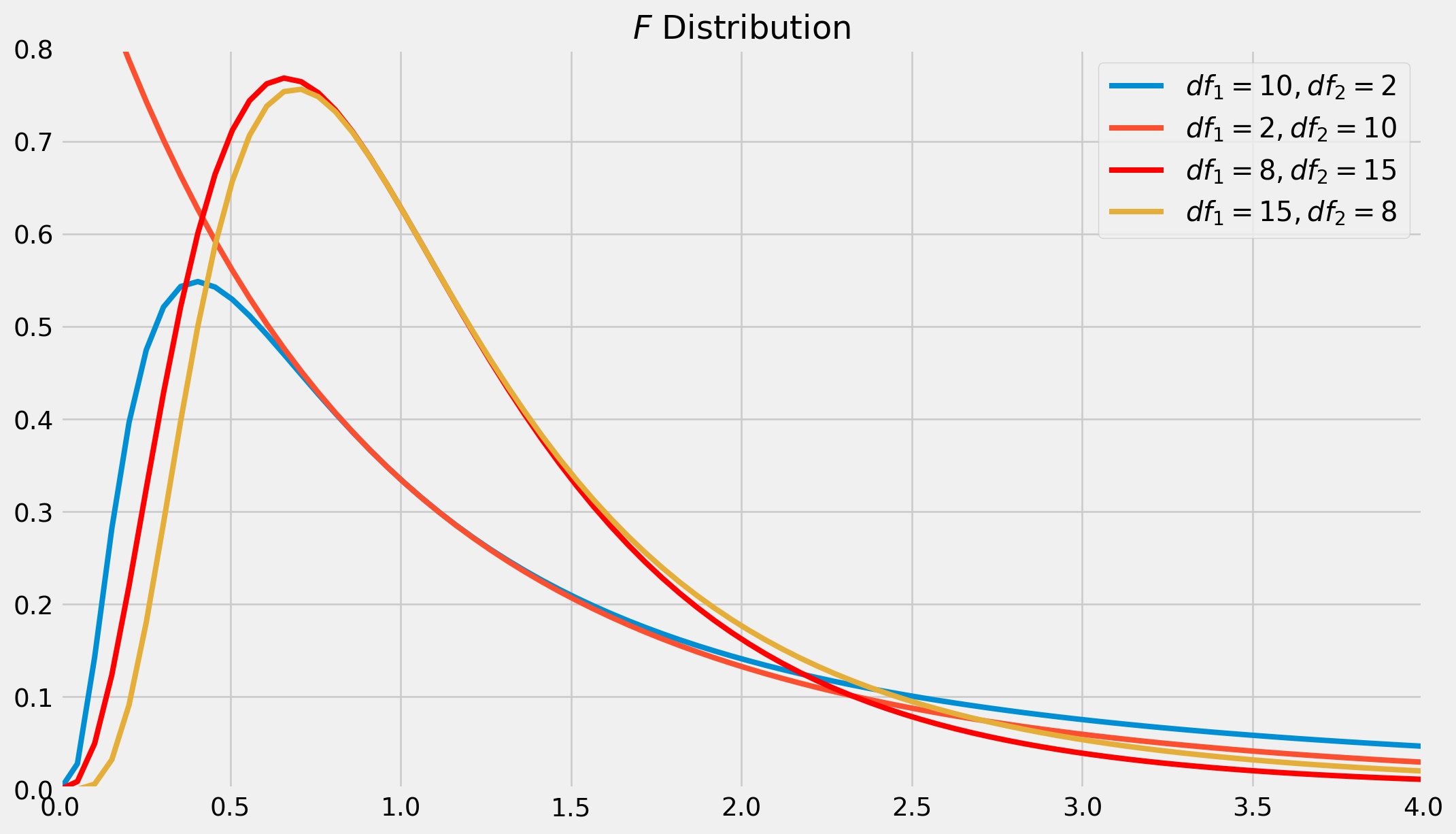
Single Restriction
Any linear restriction, such as \(\beta_1 = 5\), \(\beta_1 =2{\beta_2}\) can be tested, however, no loss of generality if linear restriction of \(\beta_2=0\) is demonstrated.
We first take a look at single restriction, see how FWL regression can help to construct statistic tests.
The regression model is
\[ \boldsymbol{y} = \boldsymbol{X}_1\boldsymbol{\beta}_1+\beta_2\boldsymbol{x}_2+\boldsymbol{u} \]
where \(\boldsymbol{x}_2\) is an \(n\)-vector, whereas \(\boldsymbol{X}_1\) is an \(n\times (m-1)\) matrix.
Project \(\boldsymbol{X}_1\) off \(\boldsymbol{x}_2\), the FWL regression is
\[ \boldsymbol{M}_1\boldsymbol{y} = \beta_2\boldsymbol{M}_1\boldsymbol{x}_2 + \boldsymbol{M}_1\boldsymbol{u} \]
Applying OLS estimate and variance formula,
\[ \hat{\beta}_2 = [(\boldsymbol{M}_1\boldsymbol{x}_2)^T\boldsymbol{M}_1\boldsymbol{x}_2]^{-1}(\boldsymbol{M}_1\boldsymbol{x}_2)^T\boldsymbol{M}_1\boldsymbol{y}=(\boldsymbol{x}_2^T\boldsymbol{M}_1\boldsymbol{x}_2)^{-1}\boldsymbol{x}_2^T\boldsymbol{M}_1\boldsymbol{y}=\frac{\boldsymbol{x}_2^T\boldsymbol{M}_1\boldsymbol{y}}{\boldsymbol{x}_2^T\boldsymbol{M}_1\boldsymbol{x}_2}\\ \text{Var}(\hat{\beta}_2) = \sigma^2 [(\boldsymbol{M}_1\boldsymbol{x}_2)^T(\boldsymbol{M}_1\boldsymbol{x}_2)]^{-1} = \sigma^2(\boldsymbol{x}_2^T\boldsymbol{M}_1\boldsymbol{x}_2)^{-1} \]
If null hypothesis is \(\beta_2^0=0\), also assuming that \(\sigma^2\) is known. Construct a \(z\)-statistic
\[ z_{\beta_2} = \frac{\hat{\beta}_2} {\sqrt{\text{Var}(\hat{\beta}_2)}}=\frac{\frac{\boldsymbol{x}_2^T\boldsymbol{M}_1\boldsymbol{y}}{\boldsymbol{x}_2^T\boldsymbol{M}_1\boldsymbol{x}_2}}{ \sigma(\boldsymbol{x}_2^T\boldsymbol{M}_1\boldsymbol{x}_2)^{-\frac{1}{2}}} = \frac{\boldsymbol{x}_2^T\boldsymbol{M}_1\boldsymbol{y}}{\sigma(\boldsymbol{x}_2^T\boldsymbol{M}_1\boldsymbol{x}_2)^{\frac{1}{2}}} \]
However, \(\sigma\) is not likely to be known, hence we replace it with \(s\), the least square standard error estimator. Recall that
\[ s^2 =\frac{1}{n-k} \sum_{t=1}^n u_t^2 = \frac{\boldsymbol{u}^T\boldsymbol{u}}{n-k}= \frac{(\boldsymbol{M_X y})^T\boldsymbol{M_X y}}{n-k}=\frac{\boldsymbol{y}^T\boldsymbol{M_X y}}{n-k} \]
Replace the \(\sigma\) in \(z_{\beta_2}\), we obtain \(t\)-statistic
\[ t_{\beta_2} = \frac{\boldsymbol{x}_2^T\boldsymbol{M}_1\boldsymbol{y}}{s(\boldsymbol{x}_2^T\boldsymbol{M}_1\boldsymbol{x}_2)^{\frac{1}{2}}} = \left(\frac{\boldsymbol{y}^T\boldsymbol{M_X y}}{n-k}\right)^{-\frac{1}{2}}\frac{\boldsymbol{x}_2^T\boldsymbol{M}_1\boldsymbol{y}}{(\boldsymbol{x}_2^T\boldsymbol{M}_1\boldsymbol{x}_2)^{\frac{1}{2}}} \]
Of course we can also show it indeed follows the \(t\) distribution by using the definition that the ratio of standard normal variable to a \(\chi^2\) variable. However, this is unnecessary for us.
Multiple Restrictions
Multiple restrictions test can be formulated as following
\[ H_0:\quad \boldsymbol{y} = \boldsymbol{X}_1\boldsymbol{\beta_1} + \boldsymbol{u}\\ H_1:\quad \boldsymbol{y} = \boldsymbol{X}_1\boldsymbol{\beta_1} +\boldsymbol{X}_2\boldsymbol{\beta_2}+ \boldsymbol{u} \]
\(H_0\) is restricted model, \(H_1\) is unrestricted. And we denote restricted residual sum of squares as \(\text{RRSS}\), and unrestricted residual sum of squares as \(\text{URSS}\), the test statistic is
\[ F_{\beta_2}= \frac{(\text{RRSS}-\text{URSS})/r}{\text{URSS}/(n-k)} \]
where \(r=k_2\), the number of restrictions on \(\beta_2\).
Using FWL regression with \(\boldsymbol{M}_1\) and \(\text{TSS = ESS + RSS}\),
\[ \boldsymbol{M}_1\boldsymbol{y}=\boldsymbol{M}_1\boldsymbol{X}_2\boldsymbol{\beta}_2+\boldsymbol{u} \tag{FWL regression} \]
\[\begin{align} \text{URSS}& =(\boldsymbol{M_1y})^T\boldsymbol{M_1y}- \underbrace{\left[\boldsymbol{M}_1\boldsymbol{X}_2[(\boldsymbol{M}_1\boldsymbol{X}_2)^T\boldsymbol{M}_1\boldsymbol{X}_2]^{-1}(\boldsymbol{M}_1\boldsymbol{X}_2)^T\boldsymbol{y}\right]^T}_{\text{projection matrix}\ P}\boldsymbol{y}\\ &= \boldsymbol{y}^T\boldsymbol{M}_1\boldsymbol{y} -\boldsymbol{y}^T\boldsymbol{M}_1\boldsymbol{X}_2(\boldsymbol{X}_2^T\boldsymbol{M}_1\boldsymbol{X}_2)^{-1}\boldsymbol{X}^T_2\boldsymbol{M}_1 \boldsymbol{y} = \boldsymbol{y}^T\boldsymbol{M_X}\boldsymbol{y} \end{align}\]
\[ \text{RRSS} = (\boldsymbol{M}_1y)^T\boldsymbol{M}_1y = \boldsymbol{y}^T\boldsymbol{M}_1\boldsymbol{y} \]
Therefore \[ \text{RRSS}-\text{URSS}=\boldsymbol{y}^T\boldsymbol{M}_1\boldsymbol{X}_2(\boldsymbol{X}_2^T\boldsymbol{M}_1\boldsymbol{X}_2)^{-1}\boldsymbol{X}^T_2\boldsymbol{M}_1 \boldsymbol{y} \]
We have all parts of \(F\) statistic, combine them
\[ F_{\boldsymbol{\beta}_{2}}=\frac{\boldsymbol{y}^{T} \boldsymbol{M}_{1} \boldsymbol{X}_{2}\left(\boldsymbol{X}_{2}^{T} \boldsymbol{M}_{1} \boldsymbol{X}_{2}\right)^{-1} \boldsymbol{X}_{2}^{T} \boldsymbol{M}_{1} \boldsymbol{y} / r}{\boldsymbol{y}^{T} \boldsymbol{M}_{\boldsymbol{X}} \boldsymbol{y} /(n-k)} \]
In contrast, \(t\) statistic will be \[ t_{\beta_{2}}=\sqrt{\frac{\boldsymbol{y}^{\top} \boldsymbol{M}_{1} \boldsymbol{x}_{2}\left(\boldsymbol{x}_{2}^{\top} \boldsymbol{M}_{1} \boldsymbol{x}_{2}\right)^{-1} \boldsymbol{x}_{2}^{\top} \boldsymbol{M}_{1} \boldsymbol{y}}{\boldsymbol{y}^{\top} \boldsymbol{M}_{\boldsymbol{X}} \boldsymbol{y} /(n-k)}} \]
To test the equality of two parameter vectors, we modify the \(F\) test as \[ F_{\gamma}=\frac{\left(\mathrm{RRSS}-\mathrm{RSS}_{1}-\mathrm{RSS}_{2}\right) / k}{\left(\mathrm{RSS}_{1}+\mathrm{RSS}_{2}\right) /(n-2 k)} \] for example, the sample being divided into two subsamples, to compare the stability of two subsamples, this so-called Chow test is a common practice.
Asymptotic Theory
Asymptotic Theory is concerned with the distribution of estimators and test statistics as the sample size \(n\) tends to infinity.
Law of Large Numbers
The widely-known Law of Large Numbers (\(\text{LLN}\)) takes the form \[ \bar{x} = \frac{1}{n}\sum_{t=1}^nx_t \] where \(x_t\) are independent variables with its own bounded variance \(\sigma_t^2\) and a common mean \(\mu\). \(\text{LLN}\) tells that as \(n\rightarrow \infty\), then \(\bar{x} \rightarrow \mu\).
The Fundamental Theorem of Statistics can be proved with \(\text{LLN}\).
An empirical distribution function (\(\text{EDF}\)) can be expressed as \[ \hat{F}(x) \equiv \frac{1}{n} \sum_{t=1}^{n} I\left(x_{t} \leq x\right) \] where \(I(\cdot)\) is an indicator function, which takes value \(1\) when its argument is true, otherwise \(0\). To prove the Fundamental Theorem of Statistics, we invoke the \(\text{LLN}\), expand the expectation
\[\begin{aligned} \mathrm{E}\left(I\left(x_{t} \leq x\right)\right) &=0 \cdot \operatorname{Pr}\left(I\left(x_{t} \leq x\right)=0\right)+1 \cdot \operatorname{Pr}\left(I\left(x_{t} \leq x\right)=1\right) \\ &=\operatorname{Pr}\left(I\left(x_{t} \leq x\right)=1\right)=\operatorname{Pr}\left(x_{t} \leq x\right)=F(x) \end{aligned}\]It turns out that \(\hat{F}(x)\) is a consistent estimator of \(F(x)\).
Central Limit Theorems
The Central Limit Theorems (\(\text{CLT}\)) tells that \(\frac{1}{n}\) times the sum of \(n\) centered random variables will approximately follow a normal distribution when \(n\) is sufficiently large. The most well \(\text{CLT}\) is Lindeberg-Lévy \(\text{CLT}\), the quantity \[ z \equiv \frac{1}{\sqrt{n}} \sum_{t=1}^{n} \frac{x_{t}-\mu}{\sigma} \] is asymptotically distributed as \(N(0,1)\).
We won’t bother to prove them, but they are the implicit theoretical foundation when we are discussing simulation-based tests.
Bootstrapping
The bootstrapping is a computational technique for handling small size sample or any sample that doesn’t follow any known distribution.
It’s rare to see it in classical linear regression model, since the sampling distribution of coefficients follow normal distribution if disturbance terms follow normal distribution.
However, for demonstration purpose, we will show how a bootstrap test is perform. The model is a simple linear regression \[ Y_t = 5 + 6 X_t + 10u_t \] where \(u_t\sim N(0, 1)\).
Generate \(Y\) and \(X\) then pass them to a data frame.
ols_obj = lr.OlsSim(100, 2, [5, 6])bootstr_params_const, bootstr_params_1 = [], []
nr_bootstrp = 100df = pd.DataFrame(ols_obj.X)
df["y"] = ols_obj.y
df.columns = ["const", "x1", "y"]resample_size = 100Repetitively sample from the generated dataframe and estimate parameters.
fig, ax = plt.subplots(figsize=(18, 8), nrows=1, ncols=3)
for i in range(nr_bootstrp):
    df_resample = df.sample(resample_size, replace=True)
    ols_fit = smf.ols(formula="y ~ x1", data=df_resample).fit()
    bootstrap_params = ols_fit.params
    bootstr_params_const.append(bootstrap_params.iloc[0])
    bootstr_params_1.append(bootstrap_params.iloc[1])
    y_pred_temp = ols_fit.predict(df_resample["x1"])
    ax[0].plot(df_resample["x1"], y_pred_temp, alpha=0.2)
ax[0].set_title("Bootstrap Regression Plot")
ax[1].hist(bootstr_params_const, bins=30)
ax[1].set_title(r"$\beta_1$")
ax[2].hist(bootstr_params_1, bins=30)
ax[2].set_title(r"$\beta_2$")
plt.show()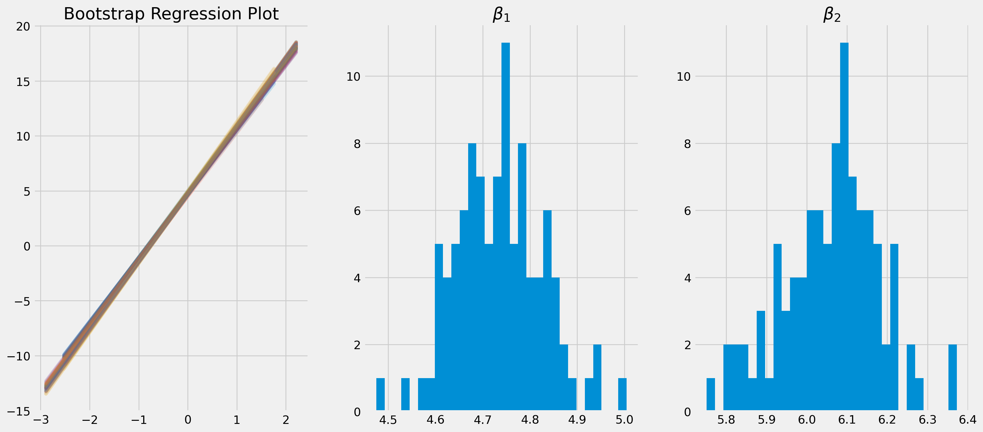
Confidence Interval
A confidence interval for some parameter \(\theta\) consists all values of \(\theta_0\) that can’t be rejected by corresponding hypothesis. If the finite-sample distribution is known, we have an exact confidence interval \([\theta_l, \theta_u]\), of which \(\theta_l\) and \(\theta_u\) represents lower and upper limit.
For instance, we have a test statistic \[ \tau\left(\boldsymbol{y}, \theta_{0}\right) \equiv\frac{\hat{\theta}-\theta_{0}}{s_{\theta}} \]
Here \(\boldsymbol{y}\) denotes the sample used to compute the particular realization of the statistic, \(\hat{\theta}\) is the estimate of \(\theta\) and \(s_\theta\) is the corresponding standard error. The confidence interval can be found by solving the equation \[ \tau(\boldsymbol{y}, \theta)=c_{\alpha} \]
where \(c_\alpha\) is the critical value with significance level \(\alpha\). Solve \[ \frac{\hat{\theta}-\theta}{s_{\theta}}=c_{\alpha} \]
Two solutions are \[ \theta_{l}=\hat{\theta}-s_{\theta} c_{\alpha} \quad \text { and } \quad \theta_{u}=\hat{\theta}+s_{\theta} c_{\alpha} \] The confidence interval is \[ [\hat{\theta}-s_{\theta} c_{\alpha},\quad \hat{\theta}+s_{\theta} c_{\alpha}] \]
To obtain critical values, it is convenient to use cumulative distribution function, e.g. the common critical value of \(t\)-statistic is \(\pm 1.96\) assuming a large degree of freedom.
sp.stats.t.ppf([0.025, 0.975], df=1000)array([-1.96233908, 1.96233908])If you wish to have the same mass on each side of the distribution, the quantiles are \(\frac{\alpha}{2}\) and \(1-\frac{\alpha}{2}\).
For a linear regression model \[ \operatorname{Pr}\left(t_{\alpha / 2} \leq \frac{\hat{\beta}-\beta}{s} \leq t_{1-(\alpha / 2)}\right)=1-\alpha \] Solve it, we get \[ \operatorname{Pr}\left(\hat{\beta}_{2}-s_{2} t_{\alpha / 2} \geq \beta_{20} \geq \hat{\beta}_{2}-s_{2} t_{1-(\alpha / 2)}\right) \]
Or more intuitively written as \[ [\hat{\beta}_{2}-s_{2} t_{1-(\alpha / 2)}, \quad \hat{\beta}_{2}+s_{2} t_{1-(\alpha / 2)}] \]
df = pd.read_excel(
    "../dataset/econometrics_practice_data.xlsx", sheet_name="US_CobbDauglas"
)
df.columns = ("Area", "Output", "Labour", "Capital")
ols_obj_fit = smf.ols(
    formula="np.log(Output) ~ np.log(Labour) + np.log(Capital)", data=df
).fit()print(ols_obj_fit.summary()) OLS Regression Results
==============================================================================
Dep. Variable: np.log(Output) R-squared: 0.964
Model: OLS Adj. R-squared: 0.963
Method: Least Squares F-statistic: 645.9
Date: Sun, 27 Oct 2024 Prob (F-statistic): 2.00e-35
Time: 17:34:27 Log-Likelihood: -3.4267
No. Observations: 51 AIC: 12.85
Df Residuals: 48 BIC: 18.65
Df Model: 2
Covariance Type: nonrobust
===================================================================================
coef std err t P>|t| [0.025 0.975]
-----------------------------------------------------------------------------------
Intercept 3.8876 0.396 9.812 0.000 3.091 4.684
np.log(Labour) 0.4683 0.099 4.734 0.000 0.269 0.667
np.log(Capital) 0.5213 0.097 5.380 0.000 0.326 0.716
==============================================================================
Omnibus: 45.645 Durbin-Watson: 1.946
Prob(Omnibus): 0.000 Jarque-Bera (JB): 196.024
Skew: 2.336 Prob(JB): 2.72e-43
Kurtosis: 11.392 Cond. No. 201.
==============================================================================
Notes:
[1] Standard Errors assume that the covariance matrix of the errors is correctly specified.ols_obj_fit.conf_int()[0]Intercept 3.090929
np.log(Labour) 0.269428
np.log(Capital) 0.326475
Name: 0, dtype: float64ols_obj_fit.conf_int()| 0 | 1 | |
|---|---|---|
| Intercept | 3.090929 | 4.684270 |
| np.log(Labour) | 0.269428 | 0.667236 |
| np.log(Capital) | 0.326475 | 0.716084 |
Full Session of Bootstrapping
df = pd.read_excel(
    "../dataset/econometrics_practice_data.xlsx", sheet_name="US_CobbDauglas"
)
df.columns = ("Area", "Output", "Labour", "Capital")
ols_obj_fit = smf.ols(
    formula="np.log(Output) ~ np.log(Labour) + np.log(Capital)", data=df
).fit()print(ols_obj_fit.summary()) OLS Regression Results
==============================================================================
Dep. Variable: np.log(Output) R-squared: 0.964
Model: OLS Adj. R-squared: 0.963
Method: Least Squares F-statistic: 645.9
Date: Sun, 27 Oct 2024 Prob (F-statistic): 2.00e-35
Time: 17:34:27 Log-Likelihood: -3.4267
No. Observations: 51 AIC: 12.85
Df Residuals: 48 BIC: 18.65
Df Model: 2
Covariance Type: nonrobust
===================================================================================
coef std err t P>|t| [0.025 0.975]
-----------------------------------------------------------------------------------
Intercept 3.8876 0.396 9.812 0.000 3.091 4.684
np.log(Labour) 0.4683 0.099 4.734 0.000 0.269 0.667
np.log(Capital) 0.5213 0.097 5.380 0.000 0.326 0.716
==============================================================================
Omnibus: 45.645 Durbin-Watson: 1.946
Prob(Omnibus): 0.000 Jarque-Bera (JB): 196.024
Skew: 2.336 Prob(JB): 2.72e-43
Kurtosis: 11.392 Cond. No. 201.
==============================================================================
Notes:
[1] Standard Errors assume that the covariance matrix of the errors is correctly specified.len(ols_obj_fit.params)3ols_obj_fit.params["Intercept"]3.88759952404164ols_obj_fit.conf_int()[0]Intercept 3.090929
np.log(Labour) 0.269428
np.log(Capital) 0.326475
Name: 0, dtype: float64ols_obj_fit.conf_int()| 0 | 1 | |
|---|---|---|
| Intercept | 3.090929 | 4.684270 |
| np.log(Labour) | 0.269428 | 0.667236 |
| np.log(Capital) | 0.326475 | 0.716084 |
formula = "np.log(Output) ~ np.log(Labour) + np.log(Capital)"
# number of bootstrap rounds
B = 2000

# placeholder matrix B rows and k columns
results_bootrp = np.zeros((B, len(ols_obj_fit.params)))

# row id range
row_id = range(0, df.shape[0])

for i in range(B):
    # this samples with replacement from rows
    this_sample = np.random.choice(
        row_id, size=df.shape[0], replace=True
    )  # gives sampled row numbers
    # Define data for this replicate:
    df_bootstrp = df.iloc[this_sample]
    # Estimate model
    params_bootstrp = smf.ols(formula, data=df_bootstrp).fit().params
    # Store in row r of results_boot:
    results_bootrp[i, :] = params_bootstrp
results_bootrp = pd.DataFrame(
results_bootrp, columns=["Intercept", "Labour", "Capital"]
)results_bootrp| Intercept | Labour | Capital | |
|---|---|---|---|
| 0 | 4.315961 | 0.554257 | 0.416290 |
| 1 | 3.829833 | 0.508452 | 0.489047 |
| 2 | 3.817793 | 0.464195 | 0.529122 |
| 3 | 3.880408 | 0.550340 | 0.450029 |
| 4 | 3.589379 | 0.468533 | 0.542215 |
| ... | ... | ... | ... |
| 1995 | 3.610902 | 0.471774 | 0.536891 |
| 1996 | 3.803365 | 0.142229 | 0.811631 |
| 1997 | 3.854466 | 0.521295 | 0.475440 |
| 1998 | 4.408160 | 0.707190 | 0.273098 |
| 1999 | 3.663214 | 0.279962 | 0.699866 |
2000 rows × 3 columns
x_range = np.arange(B)
fig, ax = plt.subplots(figsize=(18, 12), nrows=3, ncols=2)
ax[0, 0].plot(x_range, results_bootrp["Intercept"], lw=1)
ax[0, 1].hist(results_bootrp["Intercept"], bins=50, orientation="horizontal")

ax[1, 0].plot(x_range, results_bootrp["Labour"], lw=1)
ax[1, 1].hist(results_bootrp["Labour"], bins=50, orientation="horizontal")

ax[2, 0].plot(x_range, results_bootrp["Capital"], lw=1)
ax[2, 1].hist(results_bootrp["Capital"], bins=50, orientation="horizontal")
plt.show()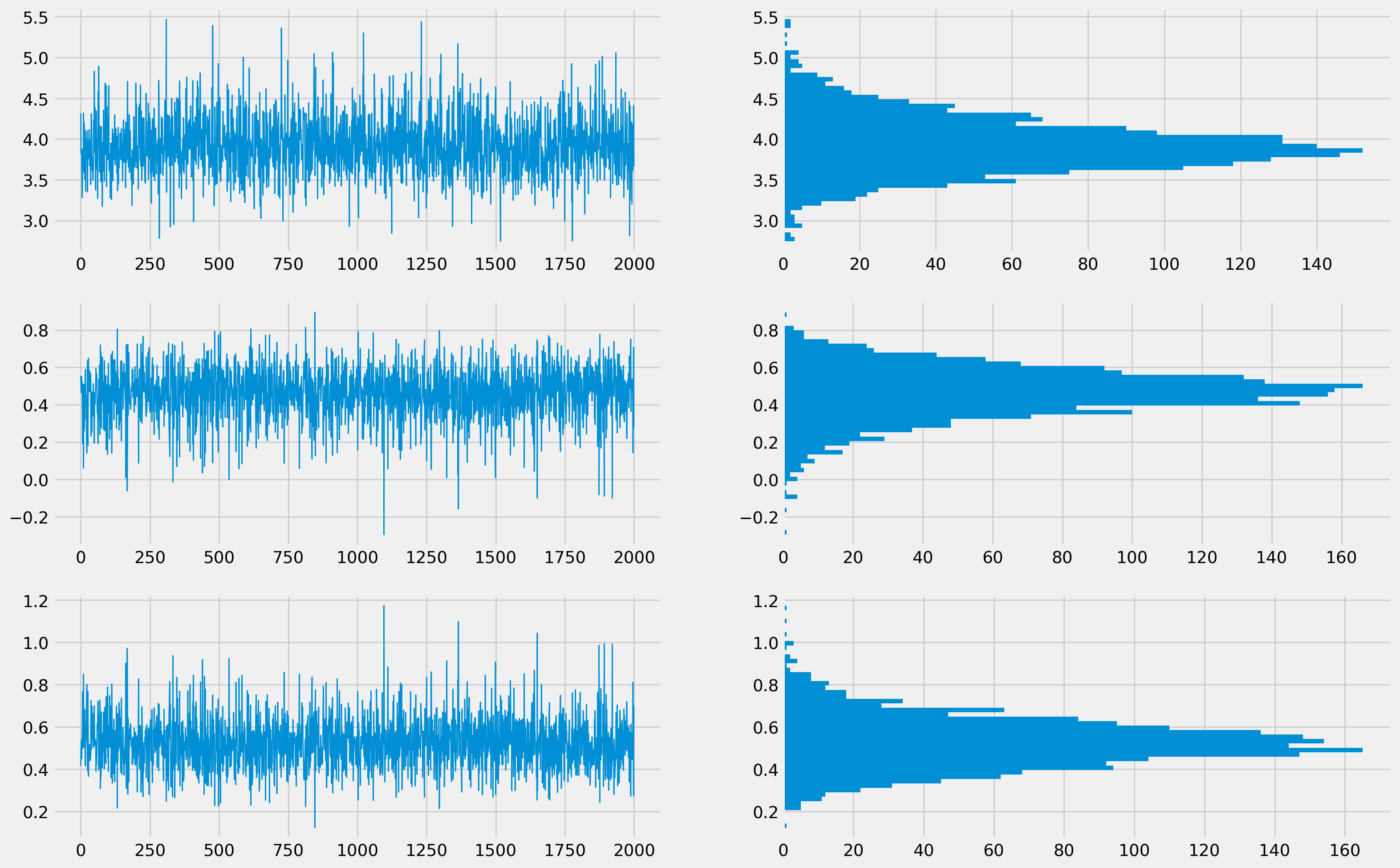
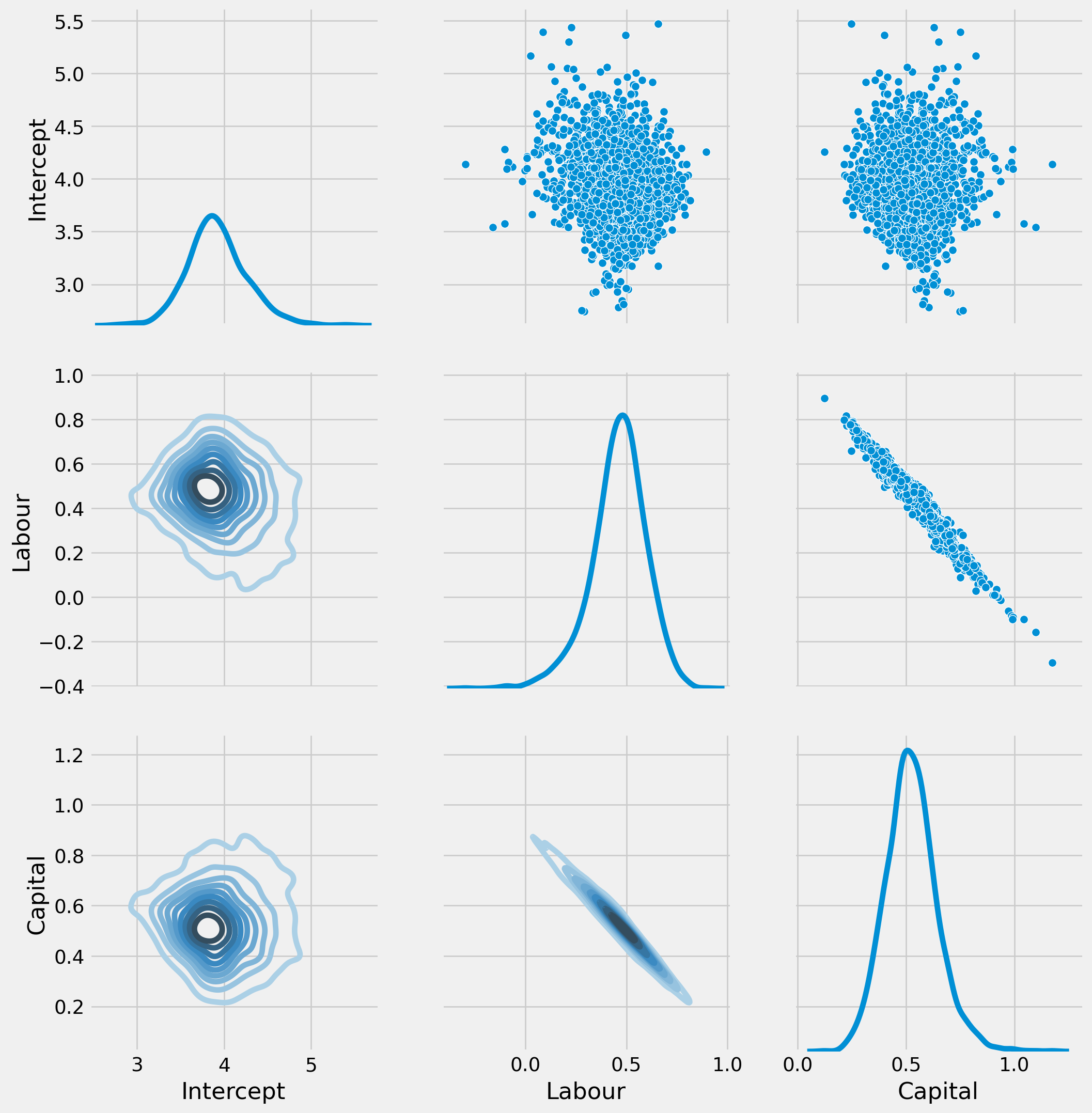
g = sns.PairGrid(results_bootrp)
g.figure.set_size_inches(12, 12)
g.map_diag(sns.kdeplot)
g.map_lower(sns.kdeplot, cmap="Blues_d")
g.map_upper(sns.scatterplot)
plt.show()